
Financial Models
Monte Carlo Simulation in Financial Modeling: How to Predict Risk and Returns
In the world of finance, uncertainty is the only certainty. Whether you’re a portfolio manager, a financial analyst, or a business owner, predicting future outcomes is a critical part of decision-making. Traditional financial models often rely on deterministic approaches, which assume fixed inputs and outputs.
However, the real world is far more complex, with countless variables influencing outcomes. This is where Monte Carlo Simulation comes into play—a powerful tool that allows you to model the uncertainty and variability inherent in financial systems.
What is Monte Carlo Simulation?
Monte Carlo simulation is a statistical technique that utilizes random sampling and statistical modeling to estimate mathematical functions and mimic the operations of complex systems. Named after the famed Monte Carlo Casino due to its inherent randomness and chance, this method has become a cornerstone in financial modeling.
The Essence of Monte Carlo Simulation
At its core, Monte Carlo simulation generates many possible scenarios for a given process, each based on random inputs. By analyzing the outcomes of these scenarios, one can obtain a probabilistic understanding of the system’s behavior. This is particularly useful in finance, where variables such as market returns, interest rates, and economic indicators are uncertain.
Historical Context
The Monte Carlo method was first introduced to finance in 1964 by David B. Hertz through his Harvard Business Review article, discussing its application in corporate finance. In 1977, Phelim Boyle pioneered simulation in derivative valuation in his seminal Journal of Financial Economics paper.
Why Use Monte Carlo Simulation in Financial Modeling?

Monte Carlo simulations have a broad spectrum of applications in finance, aiding in assessing various financial instruments and investment strategies.
1. Portfolio Valuation
Investors utilize Monte Carlo simulations to evaluate the potential future performance of their investment portfolios. Simulations can project possible portfolio values over time by modeling the random behavior of asset prices and their correlations. This assists in understanding the probability of achieving specific financial goals and making informed investment decisions.
2. Risk Assessment
Risk management is paramount in finance. Monte Carlo simulations allow analysts to quantify the impact of risk and uncertainty in financial models. Analysts can estimate the probability of different adverse outcomes by simulating various risk factors—such as market conditions, interest rates, and economic indicators—and develop strategies to mitigate potential losses.
3. Option Pricing
The valuation of complex financial derivatives, particularly options, can be challenging due to their path-dependent nature. Monte Carlo methods are extensively used to price these derivatives by simulating numerous paths that the underlying asset’s price might take and calculating the corresponding payoffs. This approach is especially beneficial for pricing exotic options that lack closed-form solutions.
4. Capital Budgeting and Project Finance
In corporate finance, Monte Carlo simulations are employed to evaluate the viability of large projects. By modeling uncertainties in cash flows, discount rates, and other variables, companies can estimate the probability distribution of a project’s net present value (NPV) or internal rate of return (IRR). This probabilistic insight aids in making informed capital budgeting decisions.
How Monte Carlo Simulation Works: A Step-by-Step Guide
Let’s break down the process of conducting a Monte Carlo Simulation in financial modeling:
- Step 1: Define the Problem and Identify Variables: Start by clearly defining the problem you want to solve. Identify the key input variables that influence the outcome. For example, if you’re modeling stock returns, the variables might include expected return, volatility, and time horizon.
- Step 2: Specify Probability Distributions: Assign probability distributions to each input variable. Common distributions include:
- Normal Distribution: For variables like stock returns.
- Lognormal Distribution: For variables that cannot be negative, such as stock prices.
- Uniform Distribution: When all outcomes are equally likely.
- Step 3: Generate Random Samples: Use a random number generator to create thousands or millions of random samples for each input variable based on their specified distributions.
- Step 4: Run Simulations: Calculate the outcome using your financial model for each set of random samples. For example, if you’re modeling portfolio returns, you might use the formula:

- Step 5: Analyze Results: Compile the results of all simulations to create a probability distribution of outcomes. Analyze key metrics such as mean, median, standard deviation, and percentiles.
- Step 6: Interpret and Make Decisions: Use the results to assess risk, identify potential outcomes, and make informed decisions. For example, you might determine the probability of achieving a target return or the likelihood of a worst-case scenario.
Example: Monte Carlo Simulation for Portfolio Returns
Let’s consider a simple example of a portfolio consisting of two assets: Stock A and Stock B. We want to simulate the future returns of this portfolio over a specific time horizon, say 10 years, using Monte Carlo simulation.
Step 1: Define the Portfolio
- Stock A: Expected annual return = 8%, Standard deviation = 15%
- Stock B: Expected annual return = 12%, Standard deviation = 20%
- Correlation between Stock A and Stock B: 0.5
- Portfolio Weights: 60% in Stock A and 40% in Stock B
Step 2: Generate Random Returns
We will generate random returns for stocks A and B based on their expected returns, standard deviations, and correlation. We can use a multivariate normal distribution to generate correlated random returns.

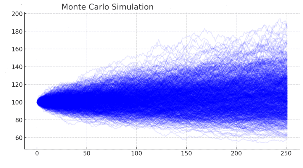
Step 3: Simulate Portfolio Growth
We can simulate the portfolio’s growth over the 10 years by compounding the annual returns.

Step 4: Analyze Results
After running the simulation, we can analyze the results to understand the distribution of possible portfolio values after 10 years.

Step 5: Interpret the Results
- Mean Final Portfolio Value: The average portfolio value after 10 years across all simulations.
- Median Final Portfolio Value: The middle value of the portfolio after 10 years, which can be less affected by extreme outcomes.
- Standard Deviation: A measure of the dispersion of the final portfolio values, indicating the risk associated with the portfolio.
Overcoming Challenges in Monte Carlo Simulation
While Monte Carlo simulation is a powerful tool for financial modeling, it comes with specific challenges that professionals must address to ensure accurate and meaningful results.
1. Choosing the Right Probability Distributions
Selecting appropriate probability distributions for input variables is crucial. A common mistake is assuming a normal distribution for all financial variables, which may not always be accurate. For example:
- Stock returns: Often modeled using a log-normal distribution rather than a normal one, as stock prices cannot be negative.
- Interest rates: May follow a mean-reverting process such as the Ornstein-Uhlenbeck model.
- Commodity prices Often exhibit skewness and kurtosis, making standard distribution assumptions problematic.
Tip: Use historical data and statistical analysis to determine the best-fit distribution for each variable.
2. Handling Correlations Between Variables
Financial variables are often interdependent. Ignoring correlations can lead to misleading results. For example, stock returns and interest rates usually exhibit inverse relationships.
Solution:
- Use a correlation matrix to model dependencies between variables.
- Employ Cholesky decomposition to generate correlated random variables in the simulation.
3. Computational Complexity and Performance
Monte Carlo simulations require running thousands or even millions of iterations, which can be computationally intensive.
Optimizations:
- Use variance reduction techniques such as antithetic variates or importance sampling to improve efficiency.
- Parallelize computations using Python’s multiprocessing or Excel’s VBA macros.
4. Interpreting Results Correctly
One of the biggest pitfalls is misinterpreting the output. Just because a particular scenario is low probability doesn’t mean it won’t happen.
Best Practices:
- Look at the tail risk (e.g., 5% worst-case scenario) instead of focusing solely on the mean or median.
- Consider running stress tests to see how the model behaves under extreme conditions.
How to Perform a Monte Carlo Simulation in Excel and Python
Using specialized functions and tools, Monte Carlo simulations can be implemented in Excel and Python.
1. Monte Carlo Simulation in Excel
Excel is an excellent tool for quick and accessible Monte Carlo simulations.
Steps:
- Define the model
- Decide on a formula or process with uncertain variables (e.g., predicting stock prices or project costs).
- Input random variables
- Use =RAND() for uniform random numbers between 0 and 1.
- Use =NORM.INV(RAND(), mean, std_dev) for normally distributed values.
- Simulate multiple scenarios
- Drag the formula down to generate thousands of random scenarios.
- Calculate key statistics
- Compute the mean, standard deviation, and other relevant metrics using Excel functions.
- Analyze results with histograms
- Use Excel’s Data Analysis ToolPak to create a histogram.
Example: Stock Price Simulation
Let’s assume a stock’s expected return is 7% with a 15% standard deviation over one year.
- In cell A1, enter the starting price: 100
- In B1, enter the formula for the next year’s price

- Drag this formula down to simulate 1000 scenarios.
- Compute:
- Mean price: =AVERAGE(B1:B1000)
- Standard deviation: =STDEV(B1:B1000)
2. Monte Carlo Simulation in Python
Python provides a more robust and flexible way to run Monte Carlo simulations using NumPy, Pandas, and Matplotlib.
Example: Stock Price Simulation

When to Use Excel vs. Python
| Feature | Excel | Python |
| Ease of use | Simple for small-scale models | Better for large-scale simulations |
| Performance | Slower with large datasets | Faster and more efficient |
| Flexibility | Limited statistical functions | More customization (NumPy, SciPy) |
| Visualization | Basic charts | Advanced plotting (Matplotlib, Seaborn) |
Practical Tips for Effective Monte Carlo Simulation
- Start Simple: Begin with a basic model and gradually add complexity as you gain confidence.
- Validate Inputs: Ensure your input variables and distributions are realistic and based on reliable data.
- Run Enough Simulations: The accuracy of your results depends on the number of simulations. Aim for at least 10,000 iterations.
- Use Sensitivity Analysis: Identify which variables impact outcomes most significantly.
- Document Assumptions: Document all assumptions and limitations of your model.
Case Study: Monte Carlo Simulation in Project Valuation Using a Financial Model
In this case study, we will evaluate a hypothetical infrastructure project using Monte Carlo simulation to estimate the Net Present Value (NPV), considering the uncertainty in key financial parameters such as initial investment, revenue growth, operating costs, and discount rate.
Project Overview
- Project Name: Green Energy Plant
- Project Duration: 10 years
- Initial Investment: $50 million
- Annual Revenue Growth Rate: 5% (±2%)
- Operating Costs: 30% of revenue (±5%)
- Discount Rate: 8% (±1%)
Monte Carlo simulation will help analyze the range of possible NPVs, providing insights into the project’s financial viability under different scenarios.
Monte Carlo Simulation Setup
To conduct the simulation:
- Define Probability Distributions for key financial inputs:
- Revenue Growth Rate: Normal distribution (mean = 5%, std. dev. = 2%)
- Operating Costs as % of Revenue: Normal distribution (mean = 30%, std. dev. = 5%)
- Discount Rate: Normal distribution (mean = 8%, std. dev. = 1%)
- Run 10,000 Simulations, calculating the NPV for each run.
- Summarize Results using statistical measures and visualizations.
Now, I will run the Monte Carlo simulation and generate the results.
Monte Carlo Simulation: NPV Distribution

Monte Carlo Simulation Results
| Growth Rate | Operating Cost % | Discount Rate | |
| count | 10000.0 | 10000.0 | 10000.0 |
| mean | 0.050040570362915315 | 0.3002260181128686 | 0.07997808603004744 |
| std | 0.019910554247468792 | 0.04968107384600725 | 0.01008925573859806 |
| min | -0.01856183610533345 | 0.11544796696907525 | 0.04046458542990874 |
| 25% | 0.03640861533085948 | 0.26678017932445197 | 0.07319111966613821 |
The Monte Carlo simulation results are now available. The histogram displays the distribution of Net Present Value (NPV) outcomes, highlighting the project’s financial uncertainty. You can also explore the summary statistics table to review key insights, such as the mean, standard deviation, and percentile values for NPV, growth rate, operating costs, and discount rate. Let me know if you need further analysis or interpretations!
Conclusion: Why Monte Carlo Simulation is a Game-Changer
Monte Carlo simulation is one of the most effective tools for risk assessment and financial forecasting. Unlike traditional static models, it provides a probabilistic view of potential outcomes, helping investors and businesses make data-driven decisions.
To simplify Monte Carlo simulations and improve accuracy, SHEETS.MARKET offers professional templates that allow you to:
- Run thousands of simulations with just a few clicks.
- Visualize risk distributions instantly.
- Customize models for your financial needs.
🚀 Save time and enhance precision—explore Sheets.Market for expert financial modeling tools today! For more insights into financial modeling, risk analysis, and Monte Carlo simulations, follow us on LinkedIn. Join the conversation and explore how these tools can support your decision-making process.